머신러닝 | 로지스틱 회귀 (Logistic Regression) 실습 | titanic 데이터 | Kaggle(캐글) 타이타닉 데이터로 생존율 예측하기 | 캐글 제출

 

타이타닉 생존 분류 문제

 

1. 타이타닉 데이터 다운받기

 

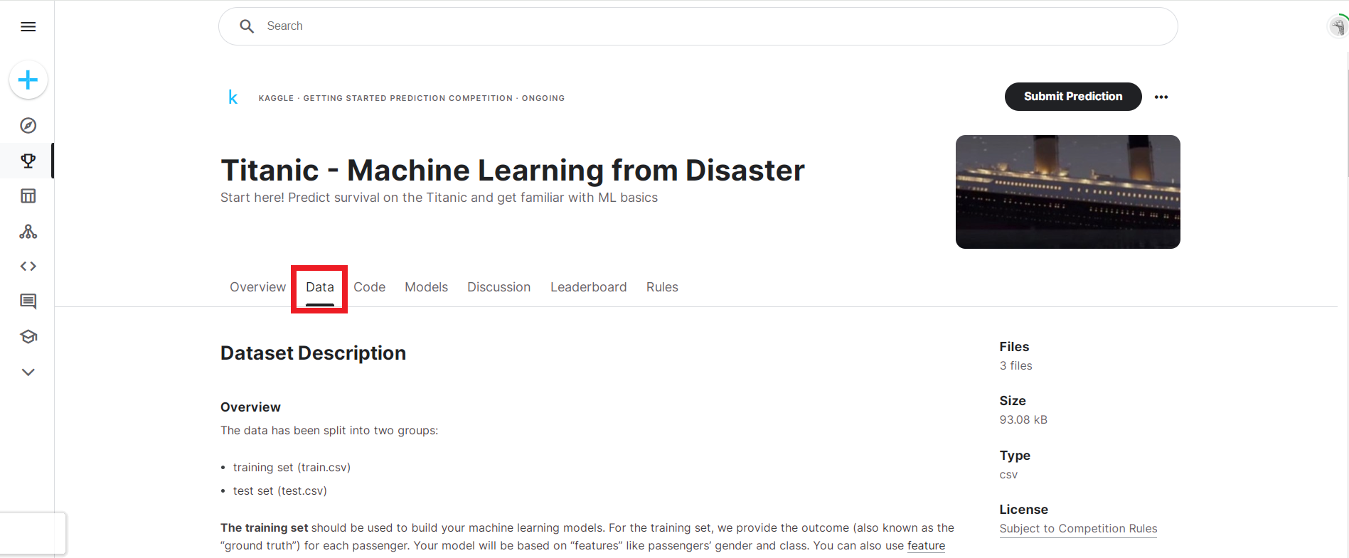
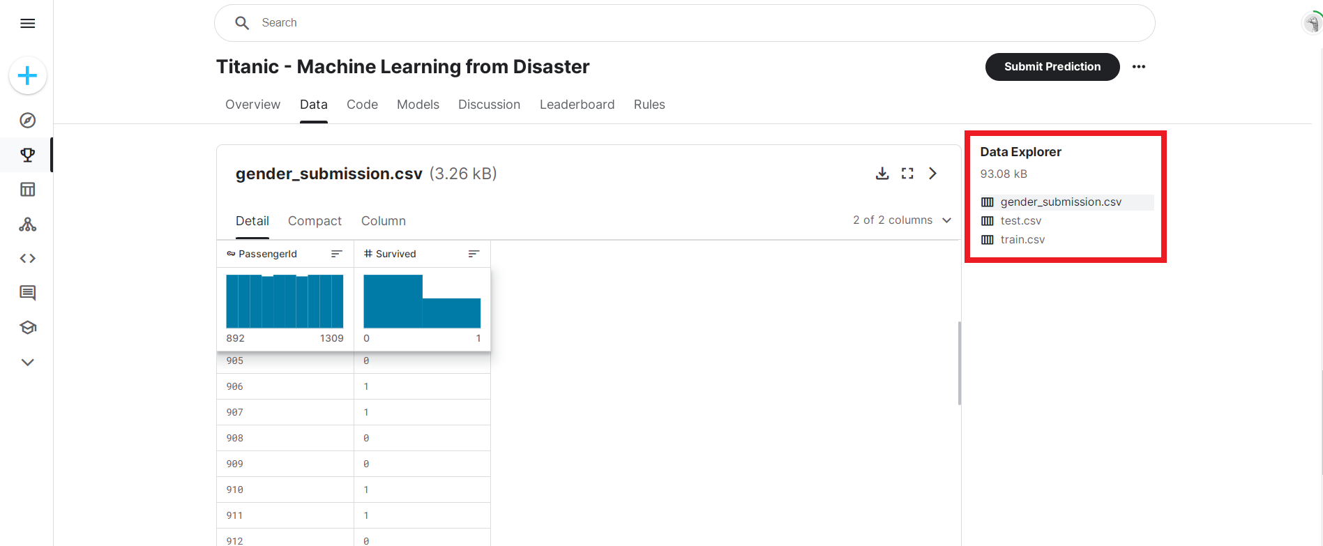
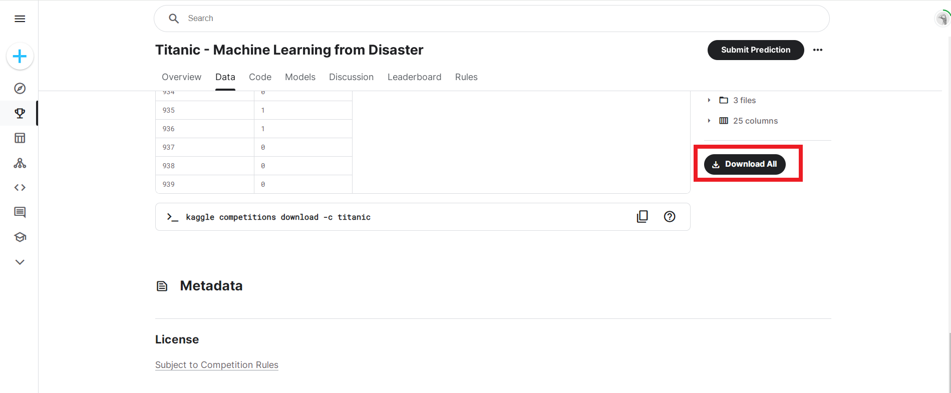
▶ Kaggle 타이타닉 예측 대회 데이터

• 주제 : 탑승한 승객 정보를 바탕으로 탑승객의 생존 유무 분류하기
• X(독립변수) : 티켓 등급, 성별, 요금 등
• Y(종속변수) : 사망(0), 생존(1)

https://www.kaggle.com/c/titanic/data

Titanic - Machine Learning from Disaster | Kaggle

Data 카테고리

 

대회 제출용.csv와 train용 데이터, test용 데이터가 있음

Download All 해주면 됨

---

2. 라이브러리 가져오기

import pandas as pd
import numpy as np
import matplotlib.pyplot as plt 
import seaborn as sns

---

3. titanic 데이터셋 구경하기

 

▶ titanic 데이터셋 안의 데이터들은 어떻게 생겼는지 살펴보기

titanic_df = pd.read_csv('titanic/train.csv')
titanic_df.head()

titanic_df.head()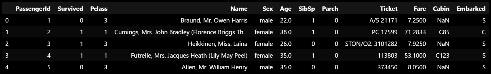

• PassengerId : 승객 아이디
• Survived : 생존 여부
• Pclass : 승선 좌석 등급
• Name : 승객 이름
• Sex : 성별
• Age : 나이
• SibSp : 형제, 배우자 동반 승선자 수
• Parch : 부모, 자녀 동반 승선자 수
• Ticket : 티켓 번호
• Fare : 승객 지불 요금
• Cabin : 선실 이름
• Embarked :  승선항 (C = Cherbourg / Q = Queenstown / S = Southhampton)

 

▶ titanic 데이터의 간략한 정보 살펴보기

titanic_df.info()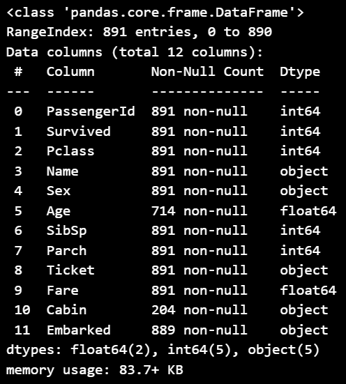

• 총 891개의 데이터
• 결측치는 Age 컬럼에 177개, Cabin 컬럼에 687개, Embarked 컬럼에 2개 존재함
• 수치형 데이터 : PassengerId, Survived, Pclass, Age, SibSp, Parch, Fare
• 문자형 데이터 : Name, Sex, Tickets, Cabin, Embarked

 

▶ titanic 데이터의 기술통계량 정보 살펴보기

: 기술통계량 정보는 수치형 데이터만 집계돼서 나오는데

include = 'all'을 넣어주면 범주형 데이터의 통계량도 확인할 수 있음

titanic_df.describe(include='all')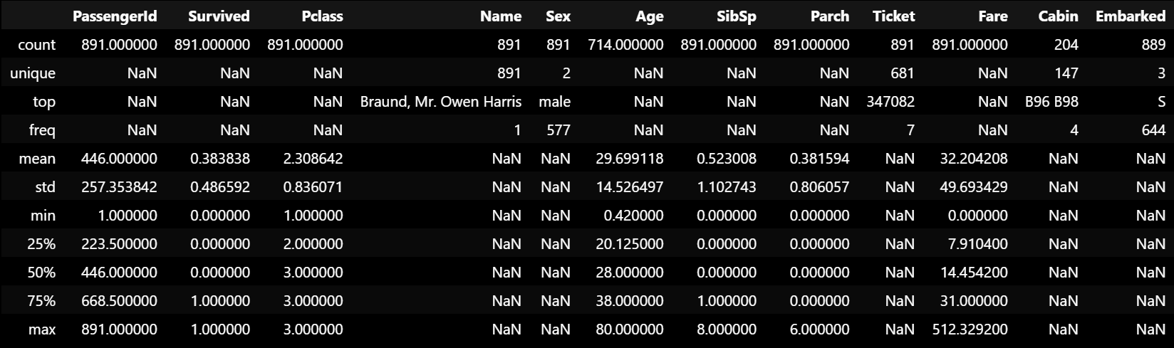

• Pclass는 1, 2, 3과 NaN값으로 이루어져 있는 것 같음
• Sex 컬럼은 두 개의 클래스로 이루어져 있고, 남성이 전체 891명 중 577명으로 약 65%를 차지하고 있음
• Age의 평균값은 29.6살
• Fare의 최댓값이 512인데 이상값이 존재하는 듯 보임
• Embarked는 총 세 개의 클래스로 이루어져 있고, S항구에서 대부분의 승객들이 탑승했음

---

4. 컬럼 간 상관관계 시각화해보기

sns.pairplot(titanic_df)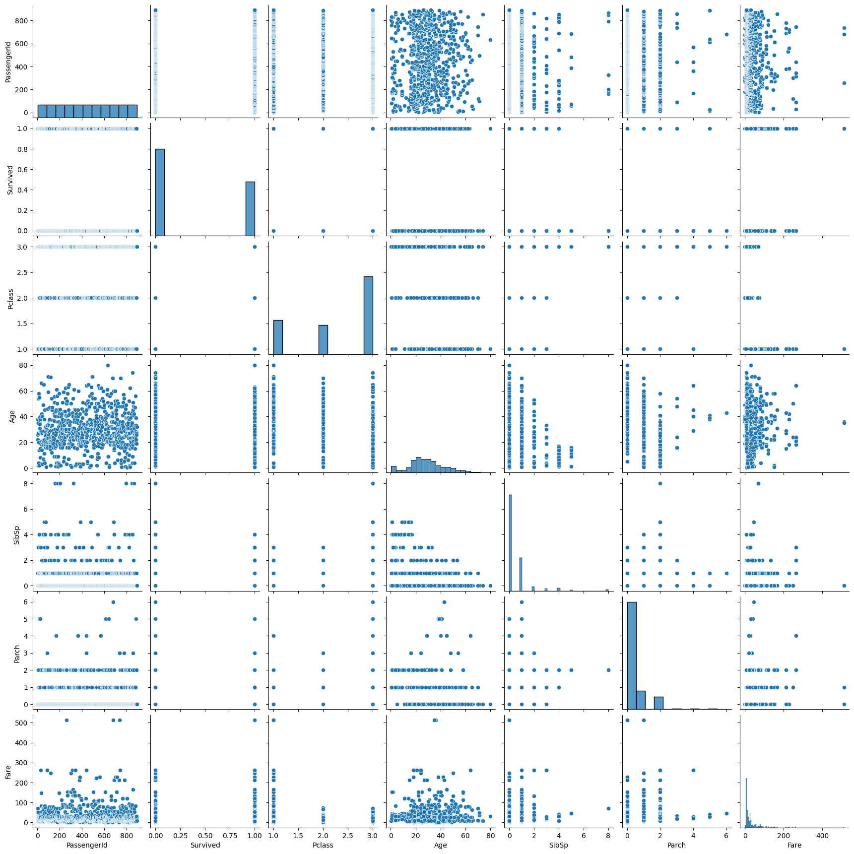

 

• Fare는 이상치가 좀 있어보임 → 전처리 필요
• 서로 선형관계를 보이고 있는 변수는 없음

---

5. titanic 데이터 전처리하기

 

5-1) Family 컬럼 만들기 (SibSp + Parch)

train_df2 = titanic_df.copy()

def get_family(df):
    df['Family'] = df['SibSp'] + df['Parch'] + 1
    return df
get_family(train_df2).head(3)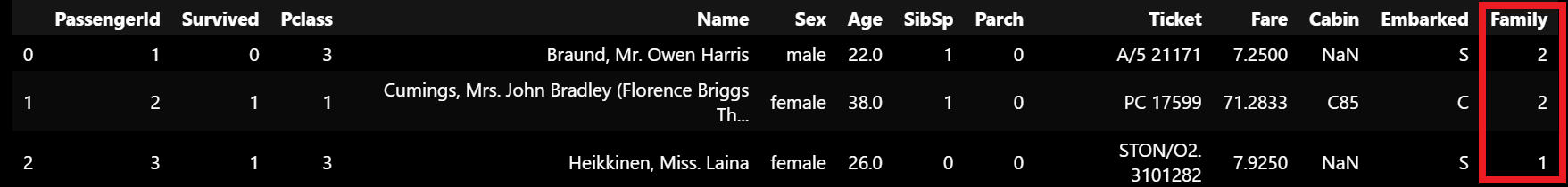

---

5-2) 데이터 이상치 처리

▶ Fare 컬럼 이상값 처리하기

train_df2 = train_df2[train_df2['Fare'] < 512]

# 이상치 제외 후 데이터프레임의 형태 확인
train_df2.shape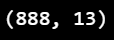

# Fare 컬럼의 기술통계량 다시 살펴보기
train_df2[['Fare']].describe()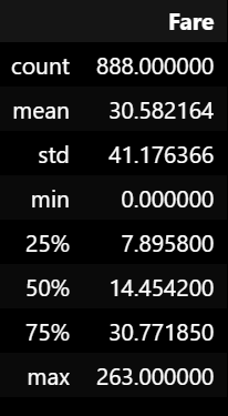

• 여전히 최댓값이 260이 넘지만, 극명한 이상치는 다 제거된 듯 함.

---

5-3) 데이터 결측치 처리

▶ Age 컬럼은 평균으로 대체

▶ Embarked 컬럼은 가장 많은 값인 'S'로 대체

def get_non_missing(df):
    Age_mean = train_df['Age'].mean()
    Fare_mean = train_df['Fare'].mean()
    df['Age'] = df['Age'].fillna(Age_mean)
    df['Embarked'] = df['Embarked'].fillna('S')
    
    # train 데이터에는 필요없지만, test 데이터에 결측치가 있으면 채워주기 위한 코드 
    df['Fare'] = df['Fare'].fillna(Fare_mean)
    
    return df
get_non_missing(train_df2).info()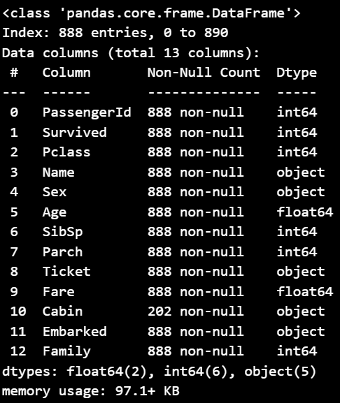

 

• Fare의 이상치를 제거한 총 888개의 데이터
• Age와 Embarked 데이터의 결측치도 다 채워진 것을 확인할 수 있음
• Cabin 컬럼은 사용하지 않을 컬럼이라 손 대지 않고 그대로 놔둠

---

6. 수치형 데이터 전처리 (스케일링)

▶ MinMaxScaler : Age, Family

▶ StandardScaler : Fare (아직 이상치가 조금 보이기 때문)

def get_numeric_sc(df):
    # sd_sc: Fare / mm_sc: Age, Family
    from sklearn.preprocessing import StandardScaler, MinMaxScaler
    sd_sc = StandardScaler()
    mm_sc = MinMaxScaler()
    
    sd_sc.fit(train_df[['Fare']])  # 학습하는 기준은 train_df이고,
    df['Fare_sd_sc'] = sd_sc.transform(df[['Fare']]) # 적용하는 곳은 들어온 df
    
    mm_sc.fit(train_df[['Age', 'Family']])  # 학습하는 기준은 train_df이고,
    df[['Age_mm_sc', 'Family_mm_sc']] = mm_sc.transform(df[['Age', 'Family']]) # 적용하는 곳은 들어온 df
    
    return df

get_numeric_sc(train_df2).describe()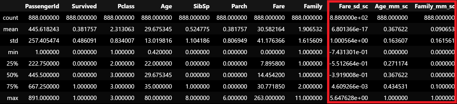

---

7. 범주형 데이터 전처리 (인코딩)

▶ LabelEncoder : Pclass, Sex

▶ OneHotEncoder : Embarked

def get_category(df):
    
    from sklearn.preprocessing import LabelEncoder, OneHotEncoder
    le = LabelEncoder()
    le2 = LabelEncoder()
    oe = OneHotEncoder()
    
    # 레이블인코딩
    le.fit(train_df[['Pclass']])
    df['Pclass_le'] = le.transform(df['Pclass'])
    
    le2.fit(train_df_2[['Sex']])
    df['Sex_le'] = le2.transform(df['Sex'])
    
    # 인덱스 리셋을 하기 위한 구문
    df = df.reset_index()
    
    # 원핫인코딩
    oe.fit(train_df[['Embarked']])
    embarked_csr = oe.transform(df[['Embarked']])  
    
    # 원핫인코딩 된 값을 데이터프레임으로 바꿔서 붙여야 함
    embarked_csr_df = pd.DataFrame(embarked_csr.toarray(), columns=oe.get_feature_names_out())
    df = pd.concat([df, embarked_csr_df], axis=1)
    
    return df

train_df2 = get_category(train_df2)

 

▶ toarray(), 희소행렬(csr)이 궁금하신 분들은 클릭!

[참고 게시글]

https://radish-greens.tistory.com/1

파이썬 scipy 희소행렬 설명 (coo, csr, dok)

---

8. 전처리가 끝난 train_df의 모습

train_df2.info()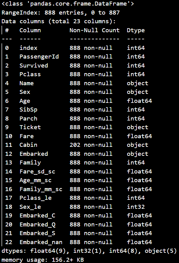

• 결측치, 이상치 처리를 완료한 총 888개의 데이터
• 수치형 데이터 : 스케일링을 마친 Fare_sd_sc, Age_mm_sc, Family_mm_sc 컬럼이 생김
• 범주형 데이터 : 인코딩을 마친 Pclass_le, Sex_le, Embarked_C, Embarked_Q, Embarked_S 컬럼이 생김

---

9. 로지스틱 모델링 시작

 

▶ 스케일링과 인코딩을 마친 컬럼들로 Survived(생존여부) 예측하기

- 로지스틱 모델의 학습 함수 만들기

def get_model(df):
    from sklearn.linear_model import LogisticRegression
    model_lor = LogisticRegression()
    X = df[['Age_mm_sc', 'Fare_sd_sc', 'Family_mm_sc', 'Pclass_le', 'Sex_le', 'Embarked_C', 'Embarked_Q', 'Embarked_S']]
    y = df[['Survived']]
    return model_lor.fit(X,y)

 

- 함수 적용

model_output = get_model(train_df2)
model_output

훈련 완료!

---

10. 모델 평가하기

 

▶ X와 y_pred 정의하기

: 로지스틱 모델이 X와 y로 훈련(훈련할 모델.fit(X,y))을 잘 했다면,

X가 y를 얼마나 잘 예측하는지(y_pred = 훈련완료된 모델.predict) 확인해보기

 

▶ 정확도(Accuracy)와 f1-score 구하기

- accuracy_score(y_true, y_pred)  

- f1_score(y_true, y_pred)

# 실제 y값과 모델이 예측한 y값을 비교해 정확도와 f1-score 확인

# 위의 y_true, y_pred는 본인들이 지정한 실제 y값, 예측 y값 변수명을 적어주면 됨

# 로지스틱 모델링 평가
from sklearn.metrics import accuracy_score, f1_score

print(accuracy_score(train_df2['Survived'], y_pred)) # 정확도
print(f1_score(train_df2['Survived'], y_pred)) # f1_score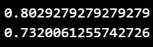

---

11. 테스트 데이터에 적용하기

 

▶ 훈련 데이터 (전처리 + 모델링)할 때 만들어놓은 함수 리스트   

• get_family(df) : SibSp컬럼 + Parch컬럼 = Family컬럼으로 합치는 함수
• get_non_missing(df) : Age컬럼, Embarked컬럼, (Fare컬럼)의 결측치를 제거해주는 함수
• get_numeric_sc(df) : 수치형 데이터 스케일링 해주는 함수
• get_category(df) : 범주형 데이터 인코딩 해주는 함수
• get_model(df) : 지정한 X변수들로 로지스틱 모델링 학습해주는 함수

---

11-1) test 데이터 함수 살펴보기

 

▶ test_df 데이터

test_df.head(3)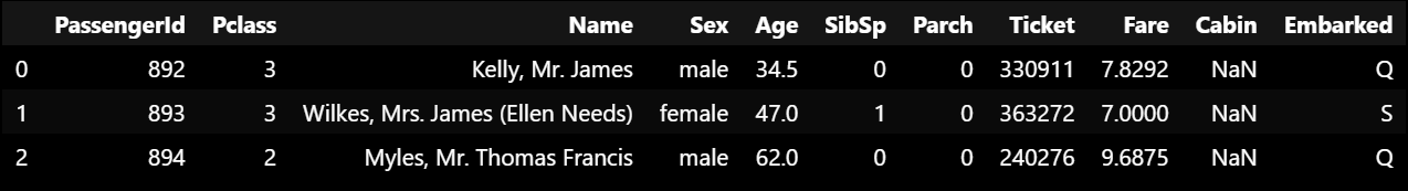

 

▶ test_df 데이터 정보

test_df.info()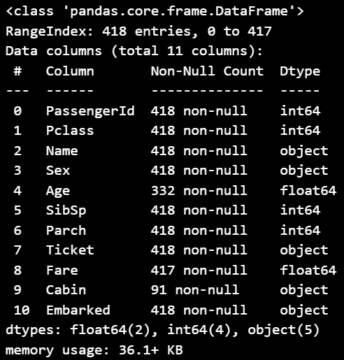

---

11-2) test 데이터 전처리

 

▶ test 데이터 전처리하기

# SibSp컬럼 + Parch컬럼 = Family컬럼 만드는 함수
test_df2 = get_family(test_df)

# Age컬럼, Embarked컬럼, (Fare컬럼)의 결측치를 제거해주는 함수
test_df2 = get_non_missing(test_df2)

# 수치형 데이터 스케일링 해주는 함수
test_df2 = get_numeric_sc(test_df2)

# 범주형 데이터 인코딩 해주는 함수
test_df2 = get_category(test_df2)

 

▶ test 데이터 전처리가 잘 됐는지 컬럼으로 확인

: 전처리가 완료된 train 데이터의 컬럼과 비교

 

- 전처리된 train_df 컬럼들

train_df2.columns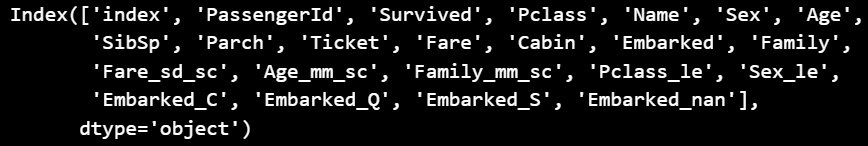

전처리 된 train_df 컬럼들

 

- 전처리된 test_df 컬럼들

test_df2.columns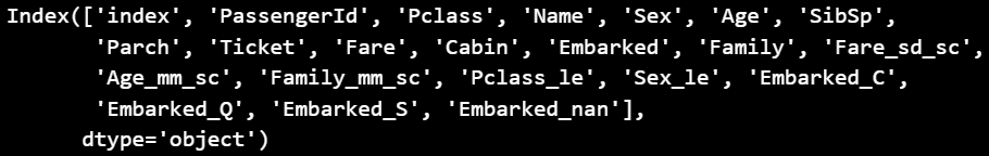

전처리된 test_df 컬럼들

---

11-3) test 데이터 모델링

 

▶ model_output 함수

: 앞서 model_output으로 train 데이터를 훈련했고, 훈련을 마친 후의 모델링의 결과를 확인할 수 있음

: 그러므로 class, coef, intercept는 다 구할 수 있음

# model_output 함수
type(model_output)

 

▶ model_output의 클래스, 가중치, 절편 확인하기

print(model_output.classes_)
print(model_output.coef_)
print(model_output.intercept_)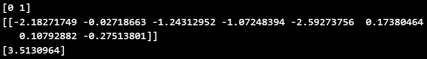

 

▶ test 데이터 X와 y_pred 값 정의

: train 데이터를 훈련해서 나온 클래스, 가중치, 절편값을 바탕으로 test 데이터의 생존율도 예측해보기

: 이 예측 정도가 얼마나 정확한지는 캐글에 제출해서 채점받을 수 있음

test_X = test_df2[['Age_mm_sc', 'Fare_sd_sc', 'Family_mm_sc', 'Pclass_le', 'Sex_le', 'Embarked_C', 'Embarked_Q', 'Embarked_S']]
y_test_pred = model_output.predict(test_X)

---

12. 캐글 제출

 

▶ gender_submission.csv 파일 열기

: 타이타닉 데이터의 train, test 데이터 다운받을 때 같이 다운 받았던 gender_sumission 파일에 결과 가져다 붙이기

# read_csv('각자 자기 컴퓨터 내에 gender_submission이 저장된 경로 붙여넣어주기')
sub_df = pd.read_csv('./gender_submission.csv')
sub_df.head(10)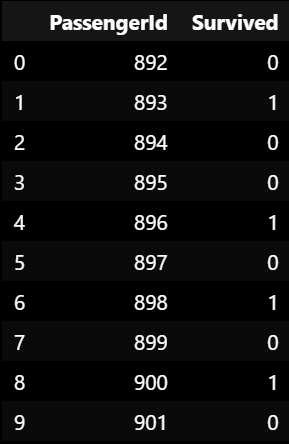

 

▶ test 데이터의 생존율을 예측한 y값(y_test_pred) 붙여넣기

sub_df['Survived'] = y_test_pred
# sub_df.head(10)

 

▶ csv파일로 저장하기

: result라는 이름의 csv 파일이 생길 것임

: 이걸 캐글의 [Submission] 카테고리에서 제출하면 됨

sub_df.to_csv('./result.csv', index = False)